안녕하세요 ! 소신입니다

Image Classification은 SeNet을 마지막으로 우선 마무리를 하고,
Object Detection 모델들의 논문 리뷰를 해보려고 합니다.
최종적으로 나만의 실시간 영상처리 모델을 구축하는 것이 목표 !
# 기존의 Object Detection
당시 Object Detection 모델의 성능은 정체되어있었는데요
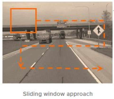
기존에는 Sliding Window 방식으로, 물체가 있을만한 곳을 하나씩 탐색하여 물체를 탐색했습니다.
이는 일일히 분류를 진행해야하기 때문에 연산량이 많고 연산시간이 오래걸려 비효율적인 방식이죠.
왜? 라고 생각하실수 있는데 Sliding window 방식은 크기가 고정되지 않아
여러 크기로도 순차적으로 계산해야하기 때문에 경우의수가 기하급수적으로 늘어나게 됩니다.
# R-CNN의 특징
R-CNN은 이러한 비효율성을 제거하고자 Region Proposal이라는 방식을 제안합니다.
Selective Search를 활용해 물체가 있을 법한 장소를 2000개 탐색하고, 이에 대해서 분류를 진행합니다.

논문에서는 물체가 있을법한 장소를 추출한 뒤, 크기에 상관없이 227x227로 이미지를 압축합니다.
그리고 이렇게 모인 이미지를 CNN을 거쳐 피쳐 벡터를 계산하고,
마지막으로 Linear SVM을 활용해 object를 분류하게 됩니다.
이렇게 하면 기존에 모든 위치를 탐색했던 방법에 비해 훨씬 빠르게 물체를 찾아낼 수 있죠
# R-CNN 모델의 학습 과정
R-CNN 모델은 Pre-Train된 CNN을 활용해 성능을 크게 향상시켰습니다.

CNN의 네트워크 구조는 ImageNet을 통해 학습된 모델을 가져오고,
맨 마지막 Fully Connected Layer만 CLASS+1로 바꿔서 Fine-Tuning 합니다.
이때 학습 데이터는 위와 같이 Region Proposal을 거쳐 227x227로 압축된 이미지가 됩니다.
Fine Tuning한 모델을 통해 추출한 4096 길이의 Feature Vector를 Linear SVM으로 Object를 분류하게 됩니다.
위의 과정을 거치면, 각 Region에 대한 분류 결과가 나오게 되고, Object 확률값을 Score로 가지게 됩니다.
이 때 2000개 박스 중에서, 겹치는 경우에는 이를 제거할 필요가 있습니다.
그 방법이 바로 Non-Maximum Suppresion이고, threshold (=경계값)를 통해 같은 Object로 볼건지, 다른 Object로 볼건지를 선택하게 됩니다.
IoU값은 아래와같이 교집합 / 합집합으로 계산이 가능합니다.

사실, 위의 경우에 박스의 위치나 크기가 정확하지 않을 수 있기 때문에,
Bounding Box Regression 방법을 활용해 물체를 정확하게 감쌀 수 있도록 조정해줍니다.

# Pytorch 구현
import zipfile
with zipfile.ZipFile('./val2017.zip') as data_zip:
    data_zip.extractall('./data')
with zipfile.ZipFile('./panoptic_annotations_trainval2017.zip') as data_zip:
    data_zip.extractall('./annotation')
구현이 목적이기 때문에 Train을 위한 데이터는 1GB짜리 2017 validation 데이터를 활용했습니다.
annotation도 2017년 것으로 가져왔습니다.
# Parameters

ano_dir = './annotation/annotations/panoptic_val2017.json'
root_dir = './data/val2017/'
annotation dir과 데이터가 있는 root dir을 가져와줍니다.
import pandas as pd
import json
import numpy as np
def get_items(ano_dir):
    with open(ano_dir, 'r') as f:
        temp = json.loads(''.join(f.readlines()))
    image_list = []
    ctg_df = pd.DataFrame(temp['categories']).reset_index()
    ctg_df['index'] = ctg_df['index'] + np.ones(len(ctg_df), dtype=np.int64)
    id2ctg = dict(ctg_df.set_index('index')['id'])
    ctg2id = dict(ctg_df.set_index('id')['index'])
    for a in temp['annotations']:
        image_id = a['file_name'][:-4]
        bbox = np.stack(marking['bbox'])
        labels = np.asarray([ctg2id[l] for l in marking['category_id']])
        image_list.append({'image_id':image_id, 'bbox':bbox, 'labels':labels})
    return np.asarray(image_list), id2ctg

image_list, id2ctg = get_items(ano_dir)
학습할 이미지들의 파일명과 박스 정보를 가져와 담아줍니다.
category가 1~200까지 중간중간 비는 값들이 있기 때문에, index를 초기화해 133개의 값을 가지게 하고,
index를 category로 변환할 수 있도록 id2ctg에 담아주었습니다.
# train_valid_split
from random import sample
def get_tv_idx(tl, k = 0.8):
    total_idx = range(tl)
    train_idx = sample(total_idx, int(tl*0.8))
    valid_idx = set(total_idx) - set(train_idx)
    return train_idx, list(valid_idx)

train_idx, valid_idx = get_tv_idx(len(image_list))
자체적으로 학습, 평가 셋으로 나누기위해 랜덤으로 index를 가져왔습니다.
train_list = image_list[train_idx]
valid_list = image_list[valid_idx]
각각 train, valid셋으로 나눠주고
def get_iou(bb1, bb2):
    assert bb1[0] < bb1[1]
    assert bb1[2] < bb1[3]
    assert bb2['x1'] < bb2['x2']
    assert bb2['y1'] < bb2['y2']
    x_left = max(bb1[0], bb2['x1'])
    y_top = max(bb1[2], bb2['y1'])
    x_right = min(bb1[1], bb2['x2'])
    y_bottom = min(bb1[3], bb2['y2'])
    if x_right < x_left or y_bottom < y_top:
        return 0.0
    intersection_area = (x_right - x_left) * (y_bottom - y_top)
    bb1_area = (bb1[1] - bb1[0]) * (bb1[3] - bb1[2])
    bb2_area = (bb2['x2'] - bb2['x1']) * (bb2['y2'] - bb2['y1'])
    iou = intersection_area / float(bb1_area + bb2_area - intersection_area)
    assert iou >= 0.0
    assert iou <= 1.0
    return iou
R-CNN은 Selective Search를 활용해서 Random 박스들을 가져온 뒤,
해당 이미지가 object인지 아닌지 확인하게 됩니다.
따라서, Selective Search로 추출한 이미지에 배경인지(0) Object인지 (1~133) 판단하기 위해
IoU를 계산해 겹치는 부분을 확인합니다.
import cv2
ss = cv2.ximgproc.segmentation.createSelectiveSearchSegmentation()

def SelectiveSearch(t):
    train_images=[]
    train_labels=[]

    img_id = t['image_id']
    img = cv2.imread(f'{root_dir}{img_id}.jpg')

    ss.setBaseImage(img)
    ss.switchToSelectiveSearchFast()
    ssresults = ss.process()
    # print(len(ssresults))

    imout = img.copy()
    counter = 0
    falsecounter = 0
    flag = 0
    fflag = 0
    bflag = 0
    boxes = t['bbox']
    x2 = boxes[:,0] + boxes[:,2]
    y2 = boxes[:,1] + boxes[:,3]
    boxes = np.c_[boxes, x2, y2][:,[0,4,1,5]]
    for _,result in enumerate(ssresults):
        if _ < 2000 and flag == 0:
            for i, gtval in enumerate(boxes):
                x,y,w,h = result
                iou = get_iou(gtval, {"x1":x,"x2":x+w,"y1":y,"y2":y+h})
                if counter < 30:
                    if iou > 0.70:
                        timage = imout[y:y+h,x:x+w]
                        resized = cv2.resize(timage, (224,224), interpolation = cv2.INTER_AREA)
                        train_images.append(resized)
                        train_labels.append(t['labels'][i])
                        counter += 1
                else :
                    fflag =1
                if falsecounter <30:
                    if iou < 0.3:
                        timage = imout[y:y+h,x:x+w]
                        resized = cv2.resize(timage, (224,224), interpolation = cv2.INTER_AREA)
                        train_images.append(resized)
                        train_labels.append(0)
                        falsecounter += 1
                else :
                    bflag = 1
            if fflag == 1 and bflag == 1:
                # print("inside")
                flag = 1

    return np.array(train_images, dtype=np.uint8), np.array(train_labels, dtype=np.int_)
Selective Search로 찾은 박스에 레이블링하는 함수입니다.
COCO Dataset은 기본적으로 x, y, w, h이기 때문에, x1, x2, y1, y2로 변환시킨 뒤,
Selective Search Box와 IoU를 계산해, 0.7보다 크면 positive, 즉 Object라고 보고 해당하는 라벨을 가져옵니다.
반대로, 0.3보다 작으면 배경으로 레이블링합니다.
모델은 SENet과 MobileNet을 합친 것을 사용했고,
모델의 classifier부분만 수정해줬습니다.
model = SEMobileNet(num_classes=10)
model.load_state_dict(torch.load('/content/drive/MyDrive/Study_AI/semob_10class.pth'))

for param in model.parameters():
    param.requires_grad = False

model.classifier = nn.Sequential(nn.Linear(1024, 4096),
                    nn.Linear(4096, len(id2ctg)+1))
model.cuda()
이전에 10개 class로 학습한 모델을 가져와서 다른곳은 학습이 되지 않도록 fix하고,
classifier부분만 Linear 두 개 (1024, 4096), (4096, 134)로 분류하게 됩니다.
사실 논문에선 Linear SVM을 사용했으므로, 따라하는게 맞지만,
Loss Function만 수정해주면 되는것같고, 우선 softmax로 실험을 해보았습니다.
import torch.optim as optim
# Linear SVM Loss MSE
criterion = nn.CrossEntropyLoss().cuda()
optimizer = optim.SGD(model.parameters(),lr=0.01, momentum=0.9, weight_decay=0.0005)
Linear SVM을 쓰신다면 MSE로 바꿔주시고, (이 부분은 확실하지 않습니다.)
from torchvision import transforms
train_transform = transforms.Compose([
                                      transforms.ToTensor(),
                                      transforms.RandomVerticalFlip(p=0.5),
                                      transforms.RandomHorizontalFlip(p=0.5),
])
transform을 정의한 뒤,
from tqdm.notebook import tqdm
total_loss = 0.0
tk0 = tqdm(train_list, total=len(train_list), leave=False)
# 4000장 * 60 = 12000
for idx, t in enumerate(tk0, 0):
    image_data, label_data = SelectiveSearch(t)
    inputs = torch.cat(tuple(train_transform(id).cuda().reshape(-1, 3, 224, 224) for id in image_data))
    labels = torch.Tensor(label_data).cuda()
    labels = labels.type(torch.long)

    outputs = model(inputs)
    loss = criterion(outputs, labels)
    loss.backward()
    optimizer.step()

    total_loss += loss.item()
학습합니다.
대략 4000 * 30 ~ 60장 정도를 확인하기 때문에, 학습이 굉장히 오래걸립니다.
저는 처음에 image를 Normalization해주지 않아서 gradient explosion이 발생했고,
모델 분류 결과가 nan값으로 채워지게 되었습니다.
그래서 transform으로 정규화를 해주었고, 이 결과를 통해 모델을 재학습했습니다.
# 결론
1. R-CNN은 Selective Search와 모델 학습 부분이 별개이기 때문에, 따로따로 학습 (병렬처리)가 가능하다.
(물론 순서는 Selective Search -> Train)
2. 거치는 과정이 굉장히 많기 때문에, 학습이 오래걸린다.
결과가 아직 나오지 않아서, 결과가 나오면 수정하겠습니다.
Ref.
'데이터 분석 > 딥러닝' 카테고리의 다른 글
| [Faster R-CNN] 논문 리뷰 & 구현 (Pytorch) (1) | 2020.12.30 |
|---|---|
| [SeNet] 논문 리뷰 & 구현 (Pytorch) (3) | 2020.12.22 |
| [MobileNet] 논문 리뷰 & 구현 (Pytorch) (0) | 2020.12.19 |